Curriculum

Week 6. Architecture, part I

Phase 2. The modern transformer · week 6 of 24

Learn in the app: tutor, coding problems →

Core: the residual stream and pre-norm, RMSNorm, SwiGLU and F = 8D/3, the B/L/T/S/V/D/H/F/N/K/G notation · Depth: weight tying, the geometry of RMSNorm (D3), hyper-connections and mHC · ≈ 10 h core / 19 h total

Every element of the modern block (pre-norm, RMSNorm, SwiGLU) answers a specific problem of the 2017 transformer; none of it is fashion. Without understanding why they are there, you will not be able to debug the training of a deep model (week 10) or count its parameters (week 9).

Notation (learn it by heart, every discussion uses it):

Step 1. The residual stream and where normalization goes

In plain terms. The residual stream is a shared notebook that L authors receive one after another. None of them rewrites the page; each one adds a correction. In post-norm, after every author the whole notebook is reprinted through a filter, and the error signal travels back to the first author through all L filters. Each filter multiplies it by its own factor, and the factors compound: at 0.9 per layer, after 32 layers you are left with 0.9³² ≈ 0.03. In pre-norm the filter sits only at the author's input: the author reads a normalized copy but adds the correction to the original.

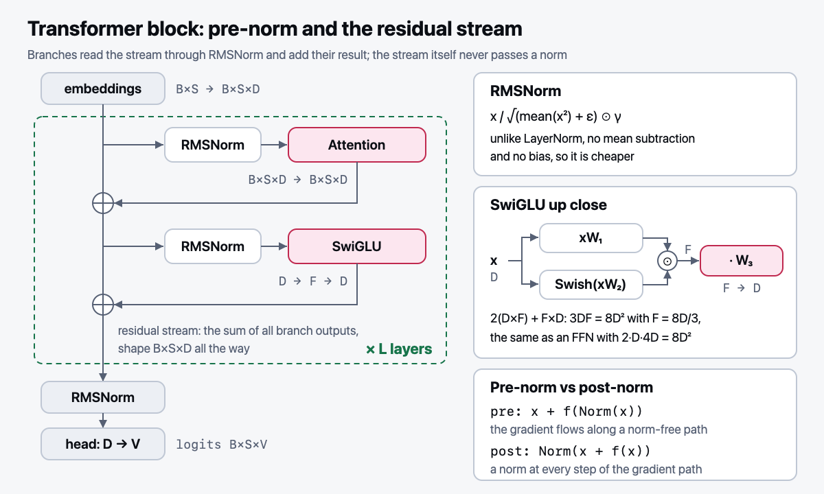
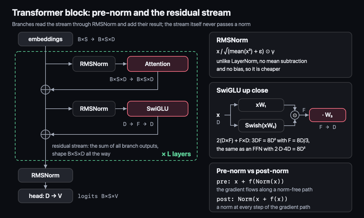
• Embeddings, the residual stream as the model's "bus": x_{l+1} = x_l + f_l(x_l). The layer's Jacobian is I + ∂f/∂x, so the gradient always has a path through the identity (the same idea as in LSTM, week 19)
• Pre-norm vs post-norm, and why everyone switched to pre-norm. Post-norm LN(x + f(x)) puts the norm right on the gradient path: at initialization the gradients of the last layers are large, and you need a long warmup (ramping the learning rate up from zero). Pre-norm x + f(LN(x)) keeps the path clean. The price: the norm of the stream grows with depth, later layers change it less and less, and a final norm is needed before the head

Clarification: addition does not guarantee information preservation. In plain terms. Adding a known constant vector c = (−2, 3) to x = (2, 1) gives (0, 4). A zero first coordinate does not prove information loss: the input is recovered as x = y − c. A counterexample needs an input-dependent update. Take a simple branch f(x₁, x₂) = (−x₁, 3): then y = x + f(x) = (0, x₂ + 3). Inputs (2, 1) and (5, 1) both produce (0, 4). The output alone cannot recover x₁, so this mapping is not invertible. This illustrates a general residual connection, not the exact form of a pre-norm transformer branch. The shared-notebook analogy does not imply immutable entries. Transformer branches are generally nonlinear, and normalization affects how they read the stream. An additive connection does not make the whole model linear. Later layers read the accumulated stream, so early contributions can affect them through intervening layers. Compare Elhage et al., Transformer Circuits. Check yourself: choose an update that preserves the first coordinate and zeroes the second.

Depth (optional). Hyper-connections and mHC: several streams instead of one.

In plain terms. Suppose there are two notebooks instead of one: streams x₁ and x₂. An author reads their mix, say 0.5x₁ + 0.5x₂, and writes the correction back into both with weights. Between authors the notebooks are mixed by a 2×2 matrix R. The ordinary residual is one stream and R = 1. Take an unconstrained R = [[1, 0.3], [0.3, 1]] and streams [1, 1]: after one layer [1.3, 1.3], and after 32 layers 1.3³² ≈ 4,400 times larger, even without the authors' corrections. Now R = [[0.7, 0.3], [0.3, 0.7]]: the entries are non-negative and every row and column sums to 1 (a doubly stochastic matrix). Streams [2, 0] become [1.4, 0.6], then [1.16, 0.84]: the sum 2 is preserved, the largest value does not grow, the streams are only averaged. A product of such matrices is doubly stochastic too, so this linear mixing chain alone does not increase the norm. This does not yet bound the full block.

• Hyper-connections (HC, Zhu et al., 2024): the stream widens to n copies of size D, X_{l+1} = R_l X_l + w_l f_l(a_l X_l). The row a_l of n weights gathers the layer input, the column w_l distributes the output, R_l (n×n) mixes the streams. The layer itself still sees a vector of size D, so the stream width becomes a separate scaling axis at almost no compute. The coefficients depend on the input: a dynamic part plus a learned static one
• The problem: unconstrained R_l multiply layer after layer, and in a deep stack training with HC often loses numerical stability; DeepSeek-V4 names this as what blocks scaling HC
• mHC (manifold-constrained HC; Xie et al., 2025): R_l is projected onto the set of doubly stochastic matrices (the Birkhoff polytope). The spectral norm of such a matrix is at most 1: mixing stretches the signal neither forward nor for the backward gradient along this branch when the matrix is fixed; products stay in the same set. When R_l depends on X_l, the full Jacobian also contains derivatives of R_l(X_l) and the nonlinear branch, so this bound does not apply to it. The projection: an exponential makes the entries positive, then columns and rows are normalized in turn (the Sinkhorn–Knopp algorithm). From [[3, 1], [1, 1]] the first round gives [[0.6, 0.4], [0.33, 0.67]], three rounds give ≈ [[0.63, 0.37], [0.37, 0.63]]. a_l and w_l go through a sigmoid: the weights are non-negative and bounded, but signed stream values can still cancel each other
• In DeepSeek-V4 (2026): n = 4 streams, 20 Sinkhorn–Knopp iterations. The static biases and gates of mHC are trained with AdamW, not Muon (week 3)

In plain terms. The vector [3, 4]: its root mean square is √((9 + 16)/2) ≈ 3.54. RMSNorm divides by it and gets [0.85, 1.13]: standard scale, same direction. LayerNorm would first subtract the mean 3.5 and get [−1, 1]: the fact that both numbers were positive is lost. Experience has shown that centering gives almost nothing but costs a separate pass over the vector.

• RMSNorm: x / √(mean(x²) + ε) ⊙ γ. How it differs from LayerNorm (no mean subtraction and no bias) and why it is cheaper: one reduction (collapsing a vector into a number) instead of two. Geometrically (D3), only for ε = 0 and before learned scale and bias: a nonzero RMSNorm output lies on a sphere of radius √D, and LayerNorm on that sphere within the hyperplane ⊥ 𝟏. With ε > 0 the norm is smaller than √D; γ changes the geometry rather than recovering the lost scale of a particular input. The learnable γ gives the model back per-dimension scale, all the way down to zeroing a dimension out

Step 2. The gated FFN

In plain terms. Swish (Swish(x) = x·σ(x), where σ is the sigmoid) is a smooth version of ReLU: a large positive number passes almost entirely, a negative one is damped almost to zero. Let F = 2, and for one token let the value be xW₁ = (3, 3) and the gate xW₂ = (2, −2). Swish of the gate: 2·σ(2) ≈ 2·0.88 = 1.76 and −2·σ(−2) ≈ −2·0.12 = −0.24. The elementwise product is (3·1.76, 3·(−0.24)) ≈ (5.28, −0.72): the same value 3 passed through amplified in the first coordinate and was almost shut off in the second. Then W₃ maps the vector back to size D. The value answers "what to pass on", the gate answers "how much".

• SwiGLU FFN: (xW₁) ⊙ Swish(xW₂), then W₃. Three matrices instead of two → F = ⅔ · 4D = 8D/3 to keep the parameter count. Derivation: 2·D·4D = 8D² = 3·D·F. It is rounded up to a multiple of 256: with D = 4096 you get 11008. One projection carries the value, the other decides through Swish how much of it to let through. This is a multiplicative interaction, and at an equal parameter count it beats the ReLU FFN in quality

• Weight tying of the input and output embeddings (one matrix for the input and for the head): saves V·D, which in GPT-2 small is about a third of all parameters. In large models the share is small, and the matrices play different roles: one reads the token, the other predicts the next one. That is why tying is often dropped there

Common mistakes

• Subtracting the mean "out of habit": you get LayerNorm without a bias, caught by test_rmsnorm_does_not_center. Normalizing along the wrong axis: test_rmsnorm_produces_unit_rms; forgetting γ: test_rmsnorm_scales_with_gamma
• Computing the norm in bf16 (16 bits: the exponent of fp32, a short mantissa; details in week 14): the sum of squares loses precision. The reference casts the input to fp32 and back
• Adding the normalized x to the stream instead of the raw one: the path through the identity disappears. There is no dedicated test: it is caught by comparing logits in week 8
• Taking F = 4D with three matrices: 1.5 times as many parameters, caught by test_swiglu_ffn_dim_is_8D_over_3 (in test_budget.py)

Code → nanolm/modules.py: RMSNorm and SwiGLU from scratch (w_gate, w_up, w_down), checked against the reference implementation. The configuration lives in ModelConfig in config.py (H, G, ffn_dim, tie_embeddings), the assembly in Block in model.py. Exercise exercises_en/modules.py, check: NANOLM_IMPL=exercises_en pytest tests/test_modules.py -k "rmsnorm or swiglu" -v.

Math (track D): D3: the geometry of LayerNorm and RMSNorm via a projector; D4: Markov, Chebyshev and norm concentration: why ‖x‖² ≈ D at initialization.

Interview question of the week: "Why did everyone switch to pre-norm, and what does it break?" A 3-minute structure: post-norm in the original → a norm on the gradient path, warmup needed → pre-norm: a path through the identity → the price: the stream's norm grows, a final norm → variants that also put a norm at the branch output (Gemma 2, OLMo 2).

Sources: Xiong et al., On Layer Normalization in the Transformer Architecture (2020); Zhang & Sennrich, RMSNorm (2019); Shazeer, GLU Variants Improve Transformer (2020); Zhu et al., Hyper-Connections (2024, ICLR 2025); Xie et al., mHC: Manifold-Constrained Hyper-Connections (2025, arXiv 2512.24880); DeepSeek-AI, DeepSeek-V4 (2026, arXiv 2606.19348).

Deeper: 05-ГЛУБИНА, section "Small additions", row "Week 6".

Week outcomes

• I can implement RMSNorm and SwiGLU that match the reference.
• I can derive F = 8D/3 from the condition that SwiGLU and a regular FFN have equal parameter counts.
• I can explain pre-norm versus post-norm in 2 minutes through the gradient path along the residual stream.
• I can name the full notation B, L, T, S, V, D, H, F, N, K, G without hints.
• I can show on two streams why mHC keeps the stream-mixing matrix doubly stochastic.

Self-check

1. What does RMSNorm remove compared with LayerNorm, and why does it have a learnable γ?
2. Why does pre-norm train more stably than post-norm?
3. What does weight tying give you, and why do large models often drop it?
4. What do hyper-connections add to the residual stream, and why does mHC require the stream-mixing matrix to be doubly stochastic?